|
Deeplabcut is one heck of a program. The GUI is pretty easy to use once you have the hang of it, and it seems very powerful. The how-to guides aren't great unfortunately, but the introductory video on using the GUI is a good step by step intro. For me I download and install it all, then open Anaconda 3 CMD with admin rights and type: activate DLC-GPU python -m deeplabcut Then it's the GUI. Some things they don't mention which are important are: 1. If it looks like nothing is happening after you click a button sometimes you have to go back to the terminal window and press the "Enter" key. 2. It's best to change the directory to C:\Deeplabcut or something like that in the CMD window and run everything there. Otherwise it can get a bit confusing where things are. 3. Make sure to install the correct (i.e. old) version of wxpython pip install -U wxPython==4.0.7.post2 Absolutely brilliant work though otherwise. 
1 Comment
Efficient Pose looks very interesting - it seems to be fast and can generate decent frame rates in "real time". I'm not confident in the accuracy claims compared to OpenPose though, and given that it can only track a single person and is nowhere near as established as Openpose it may only have a niche usefulness. Worth a look though: The article: link.springer.com/article/10.1007/s10489-020-01918-7 The github: github.com/daniegr/EfficientPose I need to check out the more advanced models on pre-recorded data, I've only played with the real-time options and frozen it up trying to run model IV. I found the installation to be a little tricky, using the method on the git page didn't work for me and I had to do a fresh install of the different packages. It can only run in Python 3.6 it seems, anything earlier or later is not compatible with the required tensorflow etc. Essentially I just opened the "requirements.txt" file and did a pip install of each one individually. For the Torch I had to remove the edition number to make it work. The Openpose demo is great:
https://github.com/CMU-Perceptual-Computing-Lab/openpose/blob/master/doc/demo_quick_start.md#faq https://github.com/CMU-Perceptual-Computing-Lab/openpose/releases The following is relevant to my computer. It’s now very simple to test and save data from openpose.
A description of the json file format is here: https://github.com/CMU-Perceptual-Computing-Lab/openpose/blob/master/doc/output.md#pose-output-format-body_25 **To close it you need to close the powershell itself. Ninjaflex might be my favourite 3D filament to print with. It is quite amazing what you can create out of this highly flexible material. We're using it to create ankle bands for the Axivity AX3 accelerometer (there's a how to guide up here for it), but you need to get your settings just right or it turns into a mess of strings. My tips for printing on a Lulzbot Taz 6 with Aerostruder are: 1. Slow the print and travel speeds right down, the slower the better. I print at 15mm/s and travel at 200mm/s. 2. Retract the filament A LOT. I use 5mm retraction, any less can cause issues. 3. I only print it with a 0.15mm layer height. Any higher and I find it can cause issues with print fails. 4. Reduce the temperature. I use 215 degrees Celsius. The default temp is too high and causes stringing for me. I've attached the curaprofile here.
Another important thing to do - for me at least - is to make sure to do at least 1 cold pull between prints. I find that if the ninjaflex cools down in the head it causes it too jam. I heat the head up to 260 degrees, pulling the ninjaflex out at around 210 degrees and extruding PLA through it at 260 for a second or two and then starting the cooldown to 70 degrees. This is annoying but now I don't get any more jams or problem prints.
Preparing a data analysis program for accelerometer data collected in people living with stroke my task is to analyse raw data collected from two wrist worn monitors, once on each arm. One of my collaborators was keen to replicate the 2D histogram methods in this paper: Hayward, K. S., Eng, J. J., Boyd, L. A., Lakhani, B., Bernhardt, J., & Lang, C. E. (2016). Exploring the Role of Accelerometers in the Measurement of Real World Upper-Limb Use After Stroke. Brain Impairment, 17(1). It seemed quite easy so I went ahead with it. However, I soon realised the problems with presenting data in this way when it is so heavily skewed. Take note of these two graphs, both of the exact same data with the only difference being the Z-axis colour bar scale and a zoom in on the Y-axis. By changing the Z-scale it makes the data look completely different, skewing in either direction depending on the settings. In the top graph it looks like vast majority of the time the person favours their left hand for movement, and that much of this occurs at bilateral magnitudes of greater than 0.05 g's. The bottom graph however shows the opposite, in that the majority of the time the person favours the right hand for movement and that almost none of the movements occur at greater than 0.05 g's. So which one is correct? 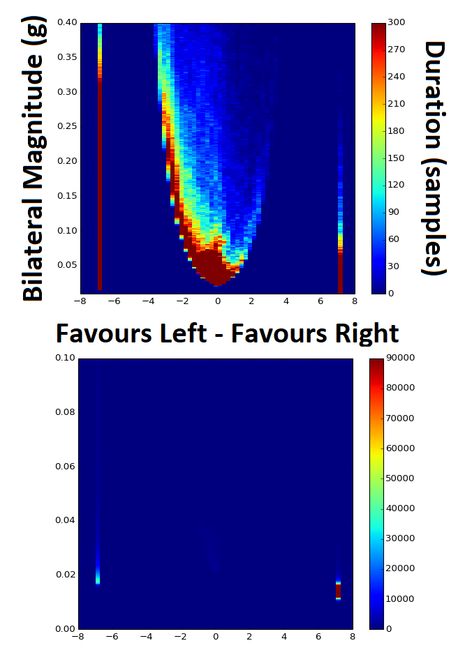 Without the 1D histogram information provided for each of the Y- and X-scale variables I now realise that these intensity charts / heat maps / 2D histograms can be a trap. The image below shows the 2D histogram with the 1D histograms for each of the axes aligned with it. This helps to tell the tale more truthfully, but adds another layer of complexity with respect to interpretation. These graphs looked simple at first glance, but as often happens with research this is not always the case. There is the potential to use a log transformed Z-scale to overcome some of this problem, but this adds in another issue in that changes in colour gradient will then be non-linear as well and therefore even more difficult to interpret. 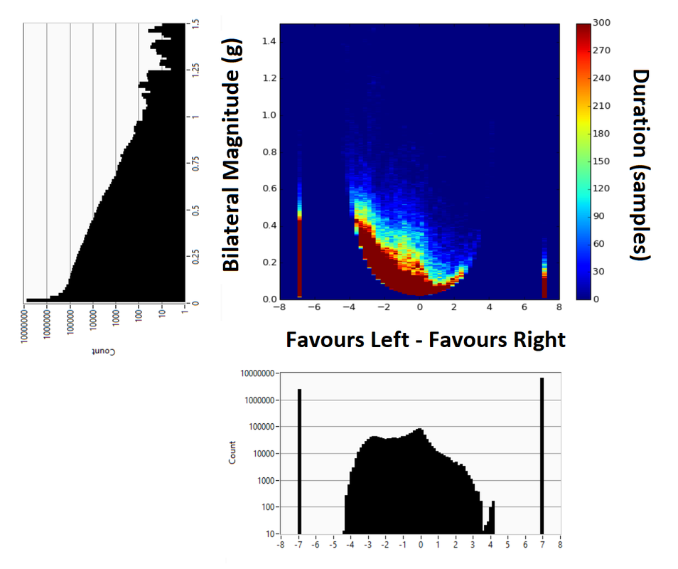 |
AuthorRoss Clark, PhD Archives
December 2022
Categories
All
|
||
 RSS Feed