A major factor in the validity of data collection is the calibration of the sensor you are using. Your calibration could be:
1. Consistently correct – if you repeat the exact same movement multiple times you will get the exact same result, and the result accurately represents the true movement.
2. Inconsistently correct – if you repeat the exact same movement multiple times you will get different results (hopefully only slightly different, but sometimes wildly different), but averaging them will give you a result that will accurately represent the movement.
3. Consistently incorrect – if you repeat the exact same movement multiple times you will get the exact same result, but the result does not accurate represent the true movement.
4. Inconsistently incorrect - if you repeat the exact same movement multiple times you will get different results, and the result does not accurate represent the true movement.
Obviously we’d prefer the first option, a consistently correct measurement system is exactly what we’re looking for. Unfortunately this is not always the case, as every sensor system has at least some error. Of the remaining options it might surprise you but we’d prefer option 3 - a system that is consistently incorrect. Just because a sensor tells you what a value is doesn’t necessarily mean it’s correct. A potentially major source of error when collecting data is poor calibration. The majority of sensors that are used to assess movement work in a reasonably simple way, they collect data in an analog or digital format which is converted into the outcome measure of interest using a calibration value. For example, many force plates collect data using strain gauges, which often export data as a raw voltage signal. This raw voltage signal itself means nothing – you need to convert it to force by knowing the relationship between change in voltage and change in force. Take for instance the following table:
As you can see from this table, when you put 100N on the force plate the voltage is equal to 1V. When you put 200N on the force plate the voltage is now equal to 2V, 300N = 3V etc. This force plate would be extremely easy to calibrate, because the relationship between voltage and force is linear (i.e. if you increase force by 100N the voltage changes by 1V). Consequently, if you had access to the raw voltage data you would simply multiply it by 100 to get your force value. For example, if the raw Voltage was 1.5V you’d be quite confident that the force is 150N.
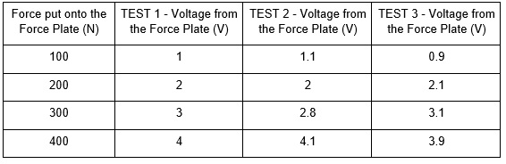
From this above example you could say that the calibration could be correct, but you don’t know how consistent it is. To find this out you’d perform multiple loading tests to assess the consistency of the calibration, similar to the following table:
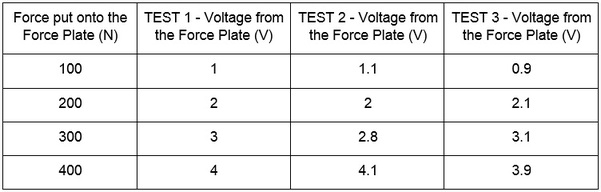
As you can see, test 1 had a perfectly linear response with a 1V increase representing a 100N increase in force. However, when you repeat the tests although you get a mostly linear response the relationship between Voltage and Force values fluctuates quite markedly. This is evident if you plot these three tests in a scatterplot with a linear fit using Excel:
What we are interested in here is the linearity – which for all tests is quite good. We know this because performing a linear fit results in quite high R2 values, which is a “goodness of fit” measure for linearity. Rounding to 2 decimal places, all three tests had a linearity of >0.99 which is a pretty good result. However, one of the issues is the consistency of the result. We can check this by examining the equation to convert the voltage value into force, and which is provided in the top right hand corner of each of the scatterplots. For test 1, which was perfectly linear, the equation is very simple:
Y=100x
This means that to get the Y-axis value (which in this case is force), you simply multiply the voltage value by 100. This is very simple and straightforward. Using the equation for test 2 is a little harder, as it is:
Y=100.82x - 2.0576
To obtain the Y-axis force value you need to multiply the voltage value by 100.82, and then subtract 2.0576. The third test equation also needs you to perform two steps, in this case it is:
Y=99.206x + 1.9841
Therefore you multiply the voltage value by 99.206, and then add 1.9841 to the value to obtain your force result.
To assess the consistency of the calibration you could check a few different voltage values with these three calibration equations. For example, if you were to obtain a reading of 3V and convert this to force using these equations your result would be 300.0N, 300.4N, and 299.6N. This is a great finding, with an extremely small amount of error. However, if you obtained a voltage of 10V your result would be 1000N, 1006.1N and 994.0N. As a percentage this is a lot more error than at 3V, with the difference between using the Test 2 and 3 calibration 1%. This is still a quite small error in the grand scheme of things, so you would be reasonably confident using these equations to obtain force values from this force plate. If you were particularly interested in the accuracy of your data, you would perform another few of these tests to make sure there wasn’t a trend or drift occurring (eg. as you perform more tests the voltage numbers get consistently higher for the same load), then average the numbers for each trial for each load and create an average calibration equation. This should get you quite accurate results when you calibrate your sensor.
Checking the Calibration of your Measurement Instruments:
This theory is all well and good, but many of the data collection systems you will use in sporting situations are calibrated in the factory and don’t give you the option to obtain the raw signal output to perform your own calibration. This can be a good thing, for example when assessing balance using centre of pressure from a force platform the manufacturer’s calibration is likely to be far more accurate then something you could perform in a field setting. I’ve attached a link to show you how this is done:
Continuing the force plate theme, although centre of pressure can be hard to calibrate the actual force calibration is quite easy. Some systems (for example the BMS force plate) include this as part of their software – and you can see examples of calibration being performed for their force plate in the following video:
As you can see in the force plate video, for this software all you need to do is put two different known loads on the force platform, and a calibration equation is created based on the raw data that the force platform records. Typically you want to use more than two loads to reduce any chance of error, but this is an easy example.
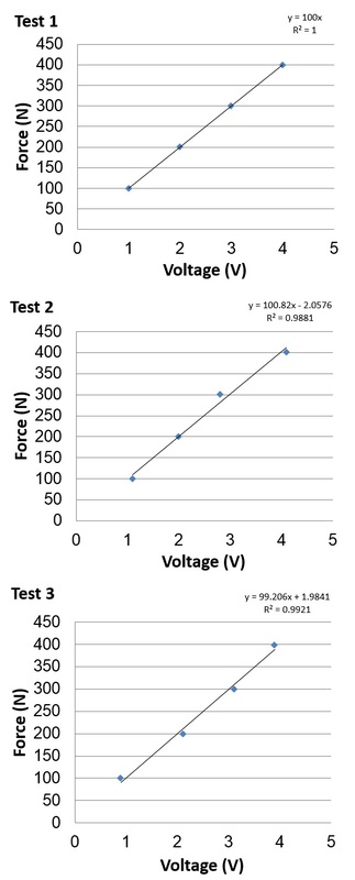
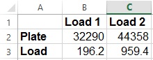
The following image is taken from the 46 second mark of that video:
The following image is taken from the 46 second mark of that video:
The known force (in kg) for the first load was 20, and for the second load was 97.8. What the force plate reported for these two loads was 32,289.69 for the first load and 44,357.74 for the second load. This results in a “Calibration Factor” of 0.0632 – but how did they get this?
It’s really quite simple, and follows the calibration examples we’ve already gone through. Here are the steps:
1. Convert the mass placed on the force plate from kilograms into Newtons, because that’s what force is reported in. This is as simple as multiplying the mass by gravity, which is approximately 9.81m/s. The two forces used in this calibration are now 196.2 and 959.4 Newtons.
2. Perform a linear fit between the numbers recorded from the force platform and the actual forces placed on the force plate. This can easily be done in Excel. Simply type the two forces (in Newtons) and the two force plate recordings into Excel in this format:
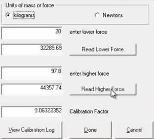
3. Now highlight the 4 cells with data in it and plot it as a scatterplot. Click on one of the data points and select “Add trendline”, then choose the option to show the equation on the chart. You will then end up with something that looks like this graph:
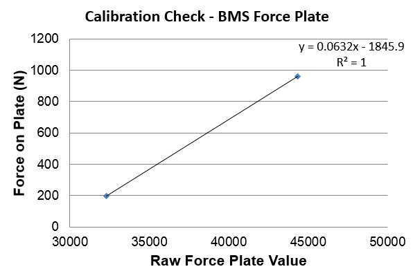
I’ve added titles and axis labels to make it easier to understand, but the important thing here is the equation “y=0.0632x – 1845.9”. As you can see, the x multiplier (0.0632) is exactly the same as the calibration factor in the BMS software (0.0632). The only difference is the number of decimal places. You’ll also see that there is a number that has to be subtracted (1845.9). In calibration terminology the multiplier is called the “scale” value and the number you either subtract or add to this value is called the “offset”
The purpose of this equation is quite simple – to get the real force value you simply multiply the raw force plate value by the scale and then subtract the offset. For example, if we multiply the raw force plate value recorded for the second load (44357.8) by this scale (0.0632) we get the value 2803.4. If we then subtract the offset from this value we get 957.5. This is the real force in Newtons, which if we divide by 9.81 to report in kilograms would give us 97.6kg. This is the same mass as the second load placed on the force plate (out by a couple of hundred grams due to rounding off errors) – and therefore you can see just how the calibration was performed.
You can apply this method to any data you collect to either calibrate it or check that it is giving you the correct values.